

Basics in Matrix Algebra
8 The Inverse
8.1 Inverting 2-by-2 Matrices
The inverse of a n-by-n matrix G is an n-by-n matrix F such that FG = In. If
this matrix
exists, we will denote it by G-1. Let us first look at an example of a 2-by-2
matrix. We have
to find coefficients a, b, c and d such that the following equation holds:
We can do this by just stating the equations for the
single components:
Solving for the coefficients of F yields:
Note that now we can solve the system of linear equations that we had in the
last lecture
by matrix-algebra operations:
Notice that this method will work for any system of linear
equations where we leave the
left-hand side unchanged (i.e. G stays as defined before) and change the vector
h on the right-hand
side. This suggests that a system of linear equations always has a unique
solution given
that the matrix on the left-hand side is invertible. In fact, this is a result
that holds for any
system of n linear equations with n unknowns, as we will see later on.
However, in general these systems do not always have a unique solution. In some
cases
they do not have any solution, in other cases they may have infinitely many
solutions. This
is related to the invertibility of the matrix on the left-hand side of the
system. Consider the
following example:
This result tells us that there are no coefficients a, b,
c and d such that DC = I. We say
that the matrix C is not invertible or singular. If you look at systems of
equations involving
the matrix C you will see that they either have no solution or infinitely many,
depending on the
vector on the right-hand side. Later, we will have a look at the general
relationship between
the invertibility of a matrix and the number of solutions of systems of linear
equations in that
matrix.
8.2 The Determinant
It turns out that the invertability of a matrix is related to its determinant.
In the case of a
2-by-2 matrix, the determinant is defined as follows:
Let us see what happens if we calculate the determinants
of the two matrices we tried to
invert before:
In fact, this result is no coincidence: If the determinant
of a matrix is 0, then it is singular,
i.e. not invertible. If the determinant is distinct from 0, then the matrix is
invertible (or
non-singular). In order to check this for higher-order matrices, however, we
need the general
definition of the determinant. In order to do this, it is useful to introduce
the following notation:
Aij is defined as the matrix that is obtained when the ith row and the jth
column of the matrix
A are deleted. An example:
With this notation at hand, we can write down a relatively
short formula for the determinant:
Note, however, that this formula requires that we know the determinants of all
terms Aij .
Note that so far, we only know them for 2-by-2 matrices (from our definition
above). Hence,
we can now calculate the determinant of a general 3-by-3 matrix:
Now that we know how to get the determinant of a 3-by-3
matrix, we could go on and
calculate the determinant of a 4-by-4 matrix, and so on. We say that this
definition of the
determinant is recursive.
You may have seen other ways of obtaining the determinant. We will not cover
them in
this course. You are free to use them throughout the course (as long as they are
correct, of
course. . .).
8.3 Systems of n Linear Equations in n Unknowns
Let us go back to the general representation of a system of n linear equations
in n unknowns
that we introduced in the last lecture:
It turns out that the determinant of G gives us a lot of
information about the number of
solutions of the system. It also depends on the nature of h: If h = 0 (i.e. all
its components
are zero) we are dealing with a homogeneous system of equations, in all other
cases (h ≠ 0,
i.e. at least one component of h is not equal zero) with an inhomogeneous system
of equations.
The number of solutions can be summarized in the following table:
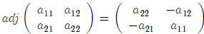
8.4 The Adjoint
In order to write down the general formula for the inverse of a matrix, we need
the concept of
the adjoint. The adjoint of a matrix A is defined as the n-by-n matrix whose row
j, column i
element is given by  (notice the change of the indeces j and i,
which amounts to
(notice the change of the indeces j and i,
which amounts to
something like a transpose). For a 2-by-2matrix this works as follows (note that
the determinant
of a 1-by-1 matrix is given by its single entry):
8.5 The Inverse of a General n-by-n Matrix
Now, we can finally write down the formula for the inverse of a general n-by-n
matrix. If the
determinant of an n-by-n matrix A is not equal to zero, then its inverse exists
and is found by
dividing the adjoint by the determinant:
8.6 Rules for Calculus with Inverses
The following rules apply for the calculus with the inverse:

9 Derivatives with Respect to Vectors
To find the minimum (or the maximum) of some function that contains a vector, we
will often
be interested in the derivative of this function with respect to every single
component of the
vector. We define the derivative of a (scalar-valued) function with respect to a
column vector
as the collection of all these derivatives in a single vector:
A very simple function of a vector x is its product with
another vector a. We can get the
derivative of this function by multiplying out and then taking the derivatives
with respect to
the single components of x:
It gets a bit more complicated if we take the derivative
of a quadratic form x'Ax. Let us
derive the general formula by looking at the simplest example where x is 2 by 2:
10 Eigenvalues and Eigenvectors
Eigenvalues of an n-by-n matrix A are values of q that solve the following
problem:
Note that we have a free choice for both q and the vector
x, as long as x ≠ 0. Let us
perform some operations on this equation to get it into the form that we are
used to:
This is a homogeneous system of n equations in n unknowns. That is, this system
can only
have a solution with x ≠ 0 if the following holds (remember the rules for the
systems of linear
equations from above!):
This condition is called the characteristic equation. Let us have a look at the
characteristic
equation if A is 2 by 2:
This is a polynomial of order 2 in the unknown q. In
general, if A is n by n then the
characteristic equation is a polynomial of order n in q. It may (or may not)
have solutions in
the space of real numbers. [Aside: If we extend our analysis to the space of
complex numbers,
however, we can always find solutions to for the characteristic equation.] The
q’s that solve the
characteristic equation are called the eigenvalues of A.
When we take one solution  back to the original problem, we can solve for the
corresponding
back to the original problem, we can solve for the
corresponding
eigenvector x. Notice that there are many possible eigenvectors related with one
eigenvalue
– since we have chosen such that the
matrix A - qI has determinant 0, this
system has
infinitely many solutions for x now. The possible eigenvectors are related to
each other: they
are multiples of one another.
Let us go through all this for the following example to get a feeling for this:
The following are important properties of eigenvalues and eigenvectors: